841
12 techniques are required to work in Excel. Entrenched in the memory!
Ecel seem strange and alarming system for people who are just starting to work with him. But it is necessary to know a little more about this tool, it becomes clear - it's incredibly easy to use. 12 These techniques will help you to work more efficiently in Ecel. Increase your productivity and make it a real holiday - thanks to our advice is very simple! It is useful to read, even those who are well-versed in the legendary program.
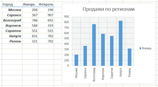
1. Add new data to a chart quickly
Select a range of new information, copy it (Ctrl + C) and insert new data in the chart (Ctrl + V).
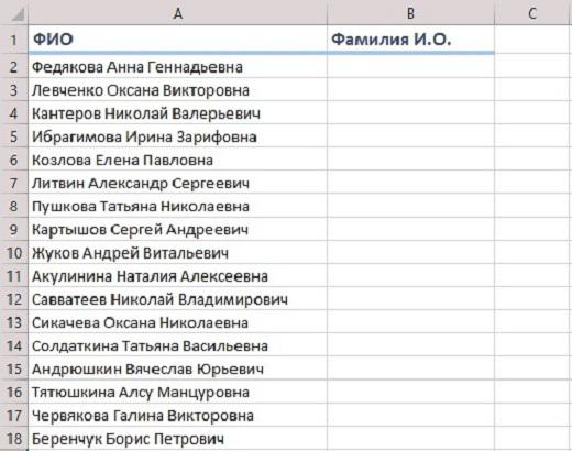
2. Immediate filling
Do you have a list of names to be converted in a shorter: for example, Levchenko Oksana - Levchenko OV Start writing the desired text in the adjacent column by hand. After 2 rows Ecel will anticipate your action and change the remaining names on similar reductions. Press Enter, to confirm the command.
3. Copiers without violating formats
Marker autocomplete - a thin black cross in the bottom right corner of the cell - copies the contents of the cell, but does so in violation of the format. After drawing a black cross click on the smart tag - An icon that appears in the lower right corner of the copied region. Select "Copy only values» (Fill Without Formatting), and registration will not be spoiled!
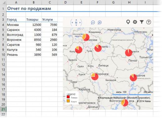
4. Display data from the table Ecel Map
Go to the "app store» (Office Store) on the "Insert» (Insert) and set out plug Bing Maps. The interactive map will show you the necessary geodata. By clicking Add, you can add a module for a direct link to the site. It will appear in the drop-down list of "My Apps» (My Apps) on the "Insert» (Insert) and will now be present on your worksheet. Now select the cells with the data and then click Show Locations module card - data will appear directly on it.
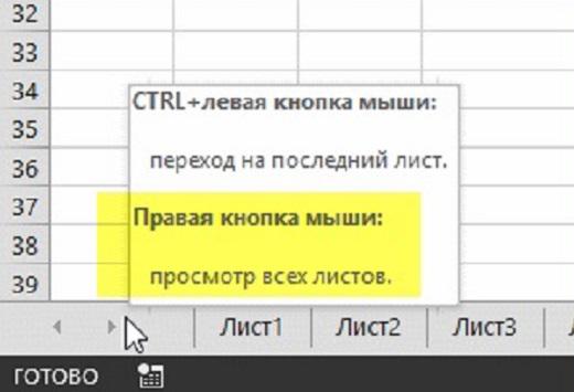
5. Transition to a new leaf quickly
See all the sheets may simply making one-click right mouse button. You can also create a list on a separate sheet of hyperlinks - all at hand.
6. Converts rows into columns and vice versa
Highlight the desired range, and you copy it. Right-click on the cell where you want to transfer data. In the context menu select "Transpose» (Transpose). Done!
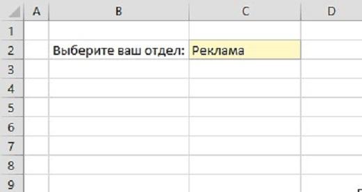
7. Do drop-down list in the cell
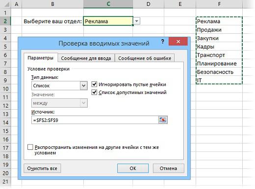
The drop-down list is needed when it is necessary to introduce certain strictly defined set of values (e.g., A or B). Select the cell or range of cells that should be a certain value. Click "Test Data" tab of the "Data» (Data - Validation).
In the dropdown list "type» (Allow), choose "List» (List). In the «» (Source) Specify the range that contains the elements of the standard version, which will subsequently fall when entering.
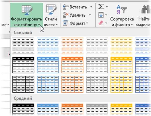
8. Make "smart" table
Select the range of data. On the "Home" click "Format as Table» (Home - Format as Table). The list will be converted to a "smart" table that contains a lot of useful features. For example, when writing up to her new rows or columns will be stretched, and introduced automatic formula will be copied to the entire column. In this table, you can add a line to the results of automatic calculation in the tab "Designer» (Design).
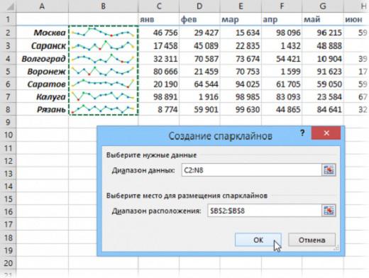
9. Sparklines Create
Sparklines - tiny figure, which reflects the dynamics of the data you entered. Click "Schedule» (Line) or "Histogram» (Columns) in the "Sparklines» (Sparklines) on the "Insert» (Insert). In the opened window, specify a range of numerical data and the cell in which you want to see Sparklines. After clicking "OK" you're done!
10. Recovers unsaved files!
If you do not save your work, which was done last time, have a chance to recover lost data. The path to recovery Ecel 2013: "File" - "Information" - "Version Control" - "Restore unsaved books» (File - Properties - Recover Unsaved Workbooks). For Ecel 10: "File" - "Last» (File - Recent) button in the lower right corner of "Restore unsaved books» (Recover Unsaved Workbooks). Open the folder in which to store temporary information.

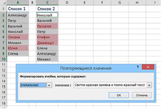
11. 2 compares the range
Hold down CTRL, you are interested in Mark columns. Select the tab "Home" - "conditional formatting" - "highlight cell rules" - "Duplicate values» (Home - Conditional formatting - Highlight Cell Rules - Duplicate Values). In the drop-down list, choose "Unique» (Unique).
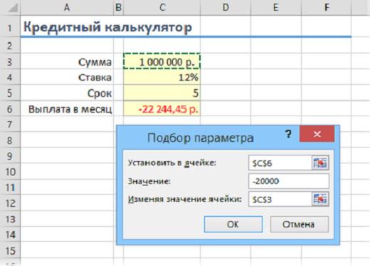
12. Pick up the results under the appropriate values
Ecel make quick and accurate adjustment of the results for you! Click on the "Insert" button "that if analysis" and then click "Seek» (Insert - What If Analysis - Goal Seek). A window appears where you can select a cell with the desired value, the desired result and the input cell that needs to change. After clicking "OK» Ecel instantly up to 0, 001 will give a hundred matching results.
Work with pleasure, and let these tips help you! Ecel - one of the world's most popular applications, and many can not imagine their activity without this program. Share useful information with your friends, it can be useful to them!
via takprosto cc
1. Add new data to a chart quickly
Select a range of new information, copy it (Ctrl + C) and insert new data in the chart (Ctrl + V).

2. Immediate filling
Do you have a list of names to be converted in a shorter: for example, Levchenko Oksana - Levchenko OV Start writing the desired text in the adjacent column by hand. After 2 rows Ecel will anticipate your action and change the remaining names on similar reductions. Press Enter, to confirm the command.

3. Copiers without violating formats
Marker autocomplete - a thin black cross in the bottom right corner of the cell - copies the contents of the cell, but does so in violation of the format. After drawing a black cross click on the smart tag - An icon that appears in the lower right corner of the copied region. Select "Copy only values» (Fill Without Formatting), and registration will not be spoiled!

4. Display data from the table Ecel Map
Go to the "app store» (Office Store) on the "Insert» (Insert) and set out plug Bing Maps. The interactive map will show you the necessary geodata. By clicking Add, you can add a module for a direct link to the site. It will appear in the drop-down list of "My Apps» (My Apps) on the "Insert» (Insert) and will now be present on your worksheet. Now select the cells with the data and then click Show Locations module card - data will appear directly on it.

5. Transition to a new leaf quickly
See all the sheets may simply making one-click right mouse button. You can also create a list on a separate sheet of hyperlinks - all at hand.

6. Converts rows into columns and vice versa
Highlight the desired range, and you copy it. Right-click on the cell where you want to transfer data. In the context menu select "Transpose» (Transpose). Done!

7. Do drop-down list in the cell
The drop-down list is needed when it is necessary to introduce certain strictly defined set of values (e.g., A or B). Select the cell or range of cells that should be a certain value. Click "Test Data" tab of the "Data» (Data - Validation).

In the dropdown list "type» (Allow), choose "List» (List). In the «» (Source) Specify the range that contains the elements of the standard version, which will subsequently fall when entering.

8. Make "smart" table
Select the range of data. On the "Home" click "Format as Table» (Home - Format as Table). The list will be converted to a "smart" table that contains a lot of useful features. For example, when writing up to her new rows or columns will be stretched, and introduced automatic formula will be copied to the entire column. In this table, you can add a line to the results of automatic calculation in the tab "Designer» (Design).

9. Sparklines Create
Sparklines - tiny figure, which reflects the dynamics of the data you entered. Click "Schedule» (Line) or "Histogram» (Columns) in the "Sparklines» (Sparklines) on the "Insert» (Insert). In the opened window, specify a range of numerical data and the cell in which you want to see Sparklines. After clicking "OK" you're done!

10. Recovers unsaved files!
If you do not save your work, which was done last time, have a chance to recover lost data. The path to recovery Ecel 2013: "File" - "Information" - "Version Control" - "Restore unsaved books» (File - Properties - Recover Unsaved Workbooks). For Ecel 10: "File" - "Last» (File - Recent) button in the lower right corner of "Restore unsaved books» (Recover Unsaved Workbooks). Open the folder in which to store temporary information.

11. 2 compares the range
Hold down CTRL, you are interested in Mark columns. Select the tab "Home" - "conditional formatting" - "highlight cell rules" - "Duplicate values» (Home - Conditional formatting - Highlight Cell Rules - Duplicate Values). In the drop-down list, choose "Unique» (Unique).

12. Pick up the results under the appropriate values
Ecel make quick and accurate adjustment of the results for you! Click on the "Insert" button "that if analysis" and then click "Seek» (Insert - What If Analysis - Goal Seek). A window appears where you can select a cell with the desired value, the desired result and the input cell that needs to change. After clicking "OK» Ecel instantly up to 0, 001 will give a hundred matching results.

Work with pleasure, and let these tips help you! Ecel - one of the world's most popular applications, and many can not imagine their activity without this program. Share useful information with your friends, it can be useful to them!
via takprosto cc


All that we say - financially. These two magic words will affect your life ...
20 soulful oriental wisdom. Every word - in the apple!