1574
Identification of rapid thermal processes
Recently I was able to complete the work in a very interesting project in the Ioffe Institute. Joffe and get enough experimental data, in order to share with you.
Physicists from the Ioffe Institute of St. Petersburg. Joffe engaged in growing gallium nitride semiconductor structures that possess a good indicator velocity of charge carriers in the transition and the high coefficient of thermal conductivity. The growth process of this structure is at a temperature of 1000 ° C (1273 K) and atmospheric pressure. Everything takes place in a special chamber located in a sealed zone. When growing structures entire volume of the reactor and sealed zone is filled with nitrogen. During the growth of the structure of the substrate holder is rotated at a rate of once per second. Such operation relates to the rapid thermal processes, the rate of change of temperature which ranges from a few to hundreds of degrees per second.
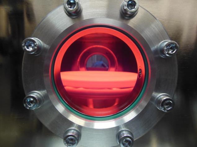
My task was to control the temperature of the graphite substrate holder by means of inductive heating.
Technical characteristics are as follows. For temperature measurement, a laser thermometer, removing the data in the center of graphite. Frequency eavesdropping 10 times per second, measuring step 1 degree. The value of the transmitted power graphite relies directly proportional to the power inductor. A generator control inductor has a digital output, which carries the voltage, current and power.
To begin, it was necessary to adjust the temperature control to the process of growth has not been strong fluctuations. Coped with this task fairly quickly, but our decision to give high quality results only at high temperatures. For other processes required to change the coefficients.
Since this work fit into the theme of my PhD, then wanted to write some clever control algorithm based on the analysis model of thermal processes. To start acquainted with the law Stefan - Boltzmann , the radiation power of a blackbody is proportional to the surface area and the fourth degree temperature. Given the convection can write an equation for thermal processes at temperatures pickup
where T - temperature, P - power, Tc - temperature of the surrounding objects, which are heated graphite own radiation, Ta - gas temperature near the point of data retrieval which performs convection, B, A1, A2 - coefficients which must be identified. For simplicity we replace all the components of the equation, which we can assume constant in the steady process and consider the following equation
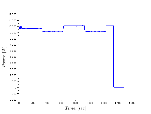
We now have available the model from which to push off with further data analysis. In the experiment, as the signal fed to meander.
If we obtain an estimate of the rate of temperature, it will be possible to make a regression model with known temperature and power control of the inductor, and calculate the coefficients in the equation.
I have long been using to work Scilab and this time decided not to change sebe.Dlya this task I chose taking the derivative of the Fourier transform. But to start working with real data, it is necessary to interpolate the measurements to obtain a uniform time axis.
Physicists from the Ioffe Institute of St. Petersburg. Joffe engaged in growing gallium nitride semiconductor structures that possess a good indicator velocity of charge carriers in the transition and the high coefficient of thermal conductivity. The growth process of this structure is at a temperature of 1000 ° C (1273 K) and atmospheric pressure. Everything takes place in a special chamber located in a sealed zone. When growing structures entire volume of the reactor and sealed zone is filled with nitrogen. During the growth of the structure of the substrate holder is rotated at a rate of once per second. Such operation relates to the rapid thermal processes, the rate of change of temperature which ranges from a few to hundreds of degrees per second.

My task was to control the temperature of the graphite substrate holder by means of inductive heating.
Technical characteristics are as follows. For temperature measurement, a laser thermometer, removing the data in the center of graphite. Frequency eavesdropping 10 times per second, measuring step 1 degree. The value of the transmitted power graphite relies directly proportional to the power inductor. A generator control inductor has a digital output, which carries the voltage, current and power.
To begin, it was necessary to adjust the temperature control to the process of growth has not been strong fluctuations. Coped with this task fairly quickly, but our decision to give high quality results only at high temperatures. For other processes required to change the coefficients.
Since this work fit into the theme of my PhD, then wanted to write some clever control algorithm based on the analysis model of thermal processes. To start acquainted with the law Stefan - Boltzmann , the radiation power of a blackbody is proportional to the surface area and the fourth degree temperature. Given the convection can write an equation for thermal processes at temperatures pickup
where T - temperature, P - power, Tc - temperature of the surrounding objects, which are heated graphite own radiation, Ta - gas temperature near the point of data retrieval which performs convection, B, A1, A2 - coefficients which must be identified. For simplicity we replace all the components of the equation, which we can assume constant in the steady process and consider the following equation
We now have available the model from which to push off with further data analysis. In the experiment, as the signal fed to meander.

If we obtain an estimate of the rate of temperature, it will be possible to make a regression model with known temperature and power control of the inductor, and calculate the coefficients in the equation.
I have long been using to work Scilab and this time decided not to change sebe.Dlya this task I chose taking the derivative of the Fourier transform. But to start working with real data, it is necessary to interpolate the measurements to obtain a uniform time axis.
 & lt; code class = & quot; matlab & quot; & gt; xx = linspace (0, round (time ($)), round (time ($)) * fs + 1) '; // New time axes' d = splin (time, temp, & quot; monotone & quot;); [Int_temp, int_temp_diff] = interp (xx, time, temp, d); & Lt; / code & gt;  pre>

It is worth noting that the variable «int_temp_diff» will contain data speeds, but they look very not show partiality.


So get to work with the data in the form of Fourier series. We will need to build additional tail data to at the end there was no gap, flip chart temperature data.


Then ask the frequency axis and do the discrete Fourier transform.
 & lt; code class = & quot; matlab & quot; & gt; fs = 10; // Sample frequency in = [int_temp; int_temp ($: - 1: 1)]; N = length (in); frequency = [0: (N-1)] / N * fs; frequency (N / 2 + 1: $) = frequency (N / 2 + 1: $) -fs; frequency = frequency '; sp = fft (in); // Fast Fourier Transform & lt; / code & gt;  pre>


At a frequency of 1 Hz is seen a clear peak, due to the fact that the substrate holder rotates with this frequency. Other sampling frequency from the fact that graphite is heated unevenly and when the rotation temperature can be increased and reduced several times.

To take the derivative of the Fourier transform, simply multiply by. After that do the inverse Fourier transform.
 & lt; code class = & quot; matlab & quot; & gt; omega = (2 *% pi *% i * frequency); tmp = sp. * omega; out = real (fft (tmp, 1)); speed_temp = out (1: N / 2); & Lt; / code & gt;  pre>


This is certainly a little better than what the function returns the derivation by cubic splines, but identification with this outstanding substandard results. Have to resort to filtering the signal.

On the advice of my friend Yura, who is engaged in the setting of ship control systems, it was decided to use the window  Blackman-Harris  for cutting unnecessary frequencies . Since in the process of growth of graphite rotates with a frequency of 1 time per second, all the oscillations with a frequency above that we are not interested. Therefore it is necessary to cut out all fluctuations above 1 [Hz]:
 & lt; code class = & quot; matlab & quot; & gt; cf = 1; // Cutoff frequency k = round (cf * N / fs); L = 2 * k + 1; a0 = 0.35875; a1 = 0.48829; a2 = 0.14128; a3 = 0.01168; for j = 0: L-1, w (j + 1) = a0 - a1 * cos (2 *% pi * j / (L-1)) + a2 * cos (4 *% pi * j / (L- 1)) - a3 * cos (6 *% pi * j / (L-1)); end h = zeros (frequency); for j = 1: 1: k + 1 h (j) = w (k + j); end h ([$: - 1: $ - k]) = h ([1: 1: k + 1]); omega = (2 *% pi *% i * frequency); omega = omega. * h; tmp = sp. * omega; out = real (fft (tmp, 1)); speed_temp = out (1: N / 2); & Lt; / code & gt;  pre>


It became much better. With that proceed to the calculation of the regression coefficients.

To get good data, you must first normalize the data vector. For the free constants in the equation must be set vector filled units.
& lt; code class = & quot; matlab & quot; & gt; constant (1: length (int_power)) = 1; norm_4_temp = norm (int_temp. ^ 4); norm_int_temp = norm (int_temp); norm_int_power = norm (int_power); norm_speed_temp = norm (speed_temp); norm_constant = norm (constant); & Lt; / code & gt; pre>
Now you can begin to find the values of the constants. Component of a matrix containing the values of the three variables and constants. In this divide each of the data vectors by its length. To obtain the coefficients must be multiplied pseudoinverse matrix normalized vector data on the rate of change of temperature.
& lt; code class = & quot; matlab & quot; & gt; LSM = [int_temp. ^ 4 / norm_4_temp, int_temp / norm_int_temp, int_power / norm_int_power, constant / norm_constant]; a0 = pinv (LSM) * speed_temp / norm_speed_temp; & Lt; / code & gt; pre>
And then you must go back to the original values of the coefficient vector.
 & lt; code class = & quot; matlab & quot; & gt; a0 (1) = a0 (1) * norm_speed_temp / norm_4_temp; a0 (2) = a0 (2) * norm_speed_temp / norm_int_temp; a0 (3) = a0 (3) * norm_speed_temp / norm_int_power; a0 (4) = a0 (4) * norm_speed_temp / norm_constant; & Lt; / code & gt;  pre>

As a result, the following value a0 = [- 1.073D-12 - 0.0029096, 0.0004617, 2.0969723], which is close to the result of  our foreign colleagues , although they used a tube heating.

Now you can proceed to the verification of the results obtained on the model. We use for this virtual simulation package Xcos Scilab. Since we have a differential equation describing the thermal process in the reactor, and all coefficients to it, then collect the following scheme.


Block «From Workspace» provide the experimental data capacity previously for this block to create a structure V. We set the sampling frequency and the time to start the simulation in the block «Clock». Long weekend of the data structure is set to input. The final simulation time should be equal to the time of the experiment. Modelling run in the program text and compare graphs of experiment and simulation.
& lt; code class = & quot; matlab & quot; & gt; V.time = xx; V.values = int_power; importXcosDiagram (& quot; D: \ PhD \ Term_model.zcos & quot;); xcos_simulate (scs_m, 4); plot (time, temp); plot (A.time, A.values, & quot; r - & quot;); & Lt; / code & gt; pre>
Here's the same thing, but for a harmonic perturbation with varying frequency.
Many thanks supervisor Arastas for their invaluable assistance and participation in the preparation of the material. Thank Zavarina Eugene for providing access to the installation and the software implementation of all experiments.
Source: habrahabr.ru/post/218297/