The logic of thinking. Part 2 Factors Bashny.Net

The previous section, we have described the most basic properties of formal neurons. Uttered that threshold adder unit accurately reproduces the nature of the spike, and linear combiner can simulate a neuron response consisting of a series of pulses. It showed that the value of the output of the linear combiner can be compared with the frequency of spikes caused by the real neuron. Now we look at the basic properties, which have such formal neurons.


Filter Hebb
Next, we will often refer to neural network models. In principle, almost all of the basic concepts of the theory of neural networks are directly related to the actual structure of the brain. The man faced with certain challenges, neural network invented many interesting designs. Evolution, through all the possible neural mechanisms that took away everything which was helpful for her. It is not surprising that so many models, devised by man, it is possible to find a clear biological prototypes. As our story does not aim even as a detailed exposition of the theory of neural networks, we touch on only the most common features needed to describe the basic ideas. For a better understanding, I highly recommend to turn to literature. For me the best textbook on neural networks - is Simon Haykin "Neural networks. Full course "(Haykin, 2006).

At the heart of many neural network models is a well-known Hebb learning rule. It was suggested physiologist Donald O. Hebb in 1949 (Hebb, 1949). In a little freestyle interpretation, it has a very simple meaning: the connection of neurons are activated together, should be strengthened, due neurons triggered regardless, should subside.
The output state of the linear combiner can be written:



If we initiate the initial values ​​of the weights of small quantities, and we will apply for a variety of input images, then nothing prevents us to try to train this neuron by Hebb rule:

where n em> - a discrete step at a time - setting the speed of learning.

Such a procedure, we increase the weight of the input, which is signaled, but do it the stronger the reaction activity of the learner neuron. If no reaction occurs then and training.

However, these weights will grow indefinitely, so you can apply for the stabilization of the normalization. For example, to divide the length of the vector derived from the "new" synaptic weights.



With this training is a redistribution of the balance between the synapses. Understand the redistribution easier if the monitor changes in the balance in two installments. First, when the neuron is active, those synapses, which receives a signal obtained additive. The weights of the synapses without signal remain unchanged. Then, the overall normalization reduces the weight of all synapses. But at the same synapses without losing the signal compared to its previous value, and synapses to redistribute signals between these losses.

Hebb's rule is nothing other than the implementation of the method of steepest descent on a surface error. In fact, we make a neuron tune out 'signals, each time shifting its weight in the opposite error, that is, in the direction antigradient. To gradient descent brought us to a local extremum, it does not slip, the speed of descent must be sufficiently small. What Hebbian learning is taken into account the smallness of the parameter.

The smallness of the learning rate parameter allows you to rewrite the previous formula in the form of a series:

If we reject the terms of the second order and above, get the right training Oia (Oja, 1982):

Positive agent responsible for Hebbian learning, and negative for the overall stability. Writing in this way allows you to feel like this training can be implemented in an analog environment without the use of the calculations, only in terms of positive and negative connections.

So, a very simple training has a wonderful property. If we gradually reduce the speed of learning, the learner neuron synapses weights converge to such values ​​that its output begins to correspond to the first principal component, which would be obtained if we used the data supplied to the relevant procedures of principal component analysis. This design is called a filter Hebb.

For example, will provide the input neuron pixel image that is comparable to each neuron synapse one point of the image. We will apply to the input neuron only two of the image - the image of vertical and horizontal lines passing through the center. One step of training - a single image, a single line, either horizontally or vertically. If these images are averaged, it will cross. But the result of training will not be like averaging. This is one of the lines. The one that is most often encountered in the submitted images. Neuron provide no averaging or crossing, and those terms that often occur together. If the images are more complex, the result may not be so visual. But it will always be a major component of it.

Education neuron leads to the fact that its balance is allocated (filter) certain way. When a new signal is applied, the more accurate the match signal and adjust the balance, the higher the response of the neuron. Trained neuron can be called neuron-detector. The image, which is described by its weights, called characteristic stimulus.

The main components
The idea of ​​the method of principal components is simple and ingenious. Suppose we have a sequence of events. Each of them we describe through its influence on the sensor, which we perceive the world. Let us assume that we have sensors, describing features. All events for us to describe the dimension of the vectors. Each component of this vector indicate the value of the corresponding ith attribute. Together, they form a random variable X em>


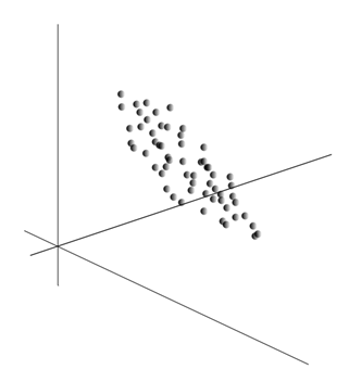
Averaging values ​​gives the expectation of a random variable X , denoted as E ( X ). If we center the data so that E ( X ) = 0, the point cloud will be concentrated around the origin.



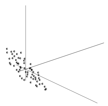
This cloud can be stretched in any direction. Having tried all possible directions, we can find along which the variance of the data will be maximum.



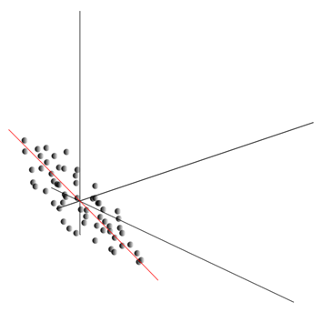
So, this direction corresponds to the first principal component. The very main component is determined by the unit vector emanating from the origin and coincides with this direction.

Further, we can find another direction perpendicular to the first component, such that the dispersion along it was also the highest among all perpendicular directions. After finding it, we obtain the second component. Then we can continue the search, specify the conditions that must be sought among the directions perpendicular to the components already found. If the original coordinates were linearly independent, so we can act again until the end of the dimension of space. Thus, we get a component A mutually arranged by what percentage of data variance they explain.

Naturally, the principal components obtained reflect intrinsic patterns our data. But there is more simple characteristics also describe the essence of the existing laws.

Assume that we have all n events. Each event is described by the vector. The components of this vector:

For each attribute can be written as it manifests itself in each of the events:

For any two features on which the description, it is possible to calculate the value indicating the degree of joint manifestations. This value is called the covariance:


It shows how much deviation from the average value of one of the signs of the manifestation of the same, with the same rejection of another sign. If the average characteristic values ​​are zero, then the covariance becomes:


If the correct covariance on standard deviations inherent characteristics, we obtain a linear correlation coefficient, also called the Pearson correlation coefficient:


The correlation coefficient has a remarkable property. It takes values ​​from -1 to 1. And 1 is a direct proportionality of the two values, and -1 indicates their inverse linear relationship.

Of all pairwise covariance signs can make the covariance matrix, which is easy to see, is the expectation of the product:

We further believe that our data is normalized, that is, have unit variance. In this case the correlation matrix coincides with the covariance matrix.

So it turns out that the main ingredient is true:

That is the main component, or, as they are called, the factors are eigenvectors of the correlation matrix. They correspond to the eigenvalues. At the same time, the greater the number of own, the greater the percentage of variance explained this factor.

Knowing all of the major components for each event is the implementation of X em> , you can burn it on the projection of the main components:

Thus, you can imagine all the original events in the new coordinates, coordinates of principal components:


Generally distinguish the search procedure the main component and the procedure of finding the basis of the factors and subsequent rotation, facilitating the interpretation of the factors, but since these procedures are ideologically close and give a similar result will be called both factor analysis.

For a fairly simple procedure of factor analysis lies very deep meaning. The fact is that if the initial signs of space - is the observed space, factors - these are signs that describe the properties and even of the world, but in the general case (if you do not agree with the observed signs) are hidden entities. That is the formal procedure of factor analysis of the phenomena observed lets go to the discovery of phenomena, although directly and invisible, but nevertheless exist in the outside world.

We can assume that our brain is actively using selection factors as one of the procedures of knowledge of the world. The factors we are able to build a new description of what is happening with us. The basis of these new definitions - the severity of what's happening in those events that match the selected factors.

Few will explain the essence of the factors at the household level. Suppose you are a manager of staff. To you get a lot of people, and on each you fill out a certain form, which record various observable data about the visitor. After reviewing my notes later, you may find that some columns have a certain relationship. For example, a haircut for men is on average shorter than women. Bald people you are likely to be found only among men, and lipstick are women only. If personal data apply to the factor analysis, it is the floor and would be one of the factors explaining the several laws. However, factor analysis allows you to find all the factors that explain the correlations in the data set. This means that in addition to the sex factor, which we can observe, and others stand out, including implicit, unobservable factors. And if the floor will appear explicitly in the questionnaire, is another important factor will be between the lines. Assessing the ability of people linked to express their thoughts, evaluating their career success by analyzing their evaluation of the diploma and the like symptoms, you will come to the conclusion that there is an overall assessment of the human intellect, which is clearly in the questionnaire is not recorded, but which explains many of its points. Assessment of intelligence - this is the hidden factor, the main component of high-cultivation effect. Obviously we do not see this component, but we fix signs, which are correlated with it. With experience, we can subconsciously on separate grounds to form an idea about the intelligence interlocutor. That procedure, which in this case uses our brain is, in fact, the factor analysis. Watching how certain phenomena occur together, the brain, using a formal procedure, highlights factors as reflected stable statistical regularities inherent in the world around us.

Selecting a set of factors
We have shown how a filter selects Hebb first principal component. It turns out that with the help of neural networks can easily obtain not only the first, but all the other components. This can be done, for example, the following method. Suppose that we have input traits. Take the linear neurons where.



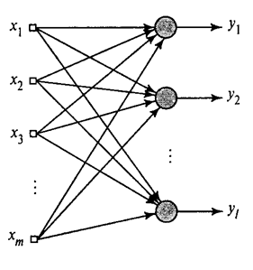
The generalized Hebb algorithm em> (Haykin, 2006)

We will teach the first neuron Hebb as a filter, so that it has allocated the first principal component. But each successive neuron will train on tap, which exclude the effect of all previous component.
The activity of neurons in step n em> is defined as


A correction to the synoptic scales like


where between 1 and 1 to. em>

For all the neurons it looks like training, a similar filter Hebb. The only difference is that each successive neuron does not see the entire signal, but only that "did not see" the previous neurons. This principle is called a reevaluation. We're actually on a limited set of components are restoring the original signal and makes the next neuron only see the rest of the difference between the original signal and the reconstructed. This algorithm is called a generalized Hebb algorithm.

In the generalized Hebb algorithm is not quite well that it is too "computing" character. Neurons should be ordered, and shortchanging their activities should be carried out strictly in sequence. It is not very matched with the principles of the cerebral cortex, each neuron at and interacts with the others, but it is off-line, and where there is no clearly defined "CPU", which would define the overall sequence of events. Because of such considerations appear more attractive algorithms, called the de-correlation algorithms.

Imagine that we have two layers of neurons Z <sub>1 sub> and Z 2 sub>. The activity of neurons in the first layer forms a kind of picture that is projected along the axons to the next layer.



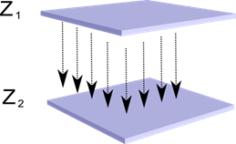
The projection of one layer to another em>

Now imagine that each neuron of the second layer has synaptic connections with all the axons coming from the first layer, if they fall within the boundaries of a certain neighborhood of the neuron (figure below). Axons entering into such an area, form the receptive field of the neuron. The receptive field of the neuron - a fragment of the total activity, which is available to him for observation. For the rest of the neuron does not exist.



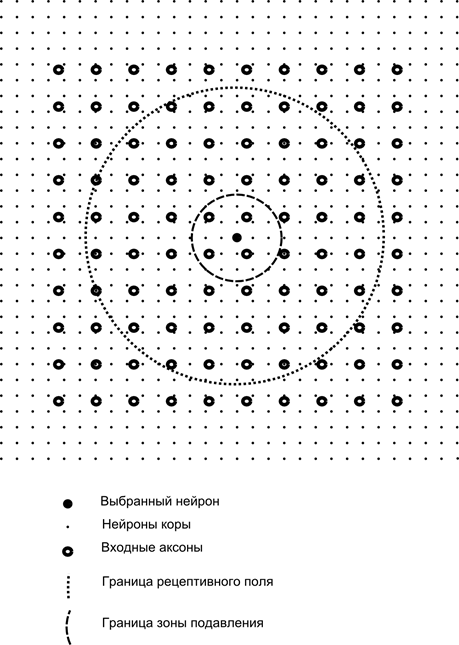
In addition to the receptive field of the neuron introduce a slightly smaller area, which we call the area of ​​suppression. Connect each neuron with its neighbors, falls into this area. Such links are called lateral or following accepted in biology terminology lateral. Make lateral inhibitory connection, that is, decrease the activity of neurons. The logic of their work - the activity of neurons inhibits the activity of all the neurons, which fall within the zone of inhibition.

Excitatory and inhibitory connections can be distributed strictly with all the axons or neurons within the boundaries of the respective regions, and can be set accidentally, such as certain densely populated center and the exponential decrease of the density of connections as the distance from it. Continuous filling easier for the simulation, a random distribution of anatomic terms of communication in real crust.

The function of neuron activity can be written:


where - the final activity - a lot of axons entering the receptive area of ​​the selected neuron - the set of neurons in the area of ​​the suppression of which gets chosen neuron - the power of the corresponding lateral inhibition, takes a negative value.

Such a function is recursive activity, because activity of the neurons is dependent on each other. This leads to the fact that a practical calculation is performed iteratively.

Education synaptic weights is similar to filter Hebb:

Lateral weight trained for anti-Hebbian rule, increasing the braking between "similar" neurons:

The essence of this design is that the Hebbian learning should result in the evolution in the balance of the neuron values ​​corresponding to the first main factors specific to the data submitted. But the neuron is able to train in the direction of a factor only when it is active.</sub>